Program of Computer Graphics
Cornell University

Andrew Butts        Stephen Marschner (advisor)

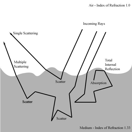
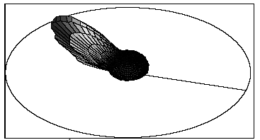
Abstract

This paper presents the results of new physics based simulations of translucent, rough surfaces. Virtual gonioreflectometry is used to collect BRDF data for a variety of material densities and surface roughnesses. Results tend to agree with prior analytical models for rough surfaces and translucent diffuse reflectors, with a few surprising inconsistencies. We employ variance-reduction techniques and implement a novel acceleration structure that yields greater accuracy without great sacrifice to simulation speed. We show several sets of plots and close-up images of the translucent material.

Introduction

Every day we distinguish between different types of materials based on their appearance. We can easily tell the difference between metal and plastic from a distance, judging by the way they tend to reflect light. We are sensitive to these differences on an unconscious level, and can easily distinguish white paint from milk, and whole milk from skim milk. Because the particular way a material reflects or transmits light is so visually significant, closely modeling these properties is a key problem in computer graphics.

Diffusely reflecting surfaces like matte paint and plastic tend to scatter reflected light in all directions, so the surface appears bright from all viewing angles. This is in contrast to shiny, mirror-like materials, which tend to scatter light with a strong directional bias.

The exact distribution of light scattered from a point on a surface is encapsulated by the bi-directional reflectance distribution function, or BRDF. Given an incoming ray of light striking a point, and any ray emanating from that same point, the BRDF yields the fraction of energy reflected.

In practice, we often approximate all diffuse surfaces by a BRDF that is simply constant for all incoming and outgoing directions. The result is a perfectly matte appearance. In reality, the materials that exhibit diffuse reflection do so because of small-scale translucency. Matte paint is composed of microscopic pigment particles suspended in a mostly transparent base such as oil. It scatters in all directions because incoming light undergoes repeated reflection off pigment particles in effectively random directions. The same is true of plastics.

We can model the BRDFs of rough-surfaced opaque materials like brushed aluminum by mathematical expressions. Such models often require statistical statements to be made about the distribution of microscopic bumps or scratches in the surface. Once the surface is characterized in this way, further statements may be made about the effect of bumps casting shadows on each other, reflecting light onto each other, or masking each other’s reflected light.

While similar analytical models exist for diffuse reflection, no attempt has been made so far to fully explore the properties of a translucent, paint-like material with an arbitrarily rough surface. This paper discusses the results of new physics based simulations of such materials.

Previous Work

Because we are concerned with translucent materials and rough surfaces, we explored work done on representations for both. Rapidly computable ad-hoc models like Lambert, Phong, and Phong variants were of little relevance. On the other hand, physically based analytical models gave us an idea of what to expect. These included the Oren-Nayar model for rough diffuse surfaces [6], the Cook-Torrance model for rough specular surfaces [1], the comprehensive He-Torrance-Sparrow-Greenberg model [4], and Koenderink, Van Doorn, Dana and Nayar’s model for “thoroughly pitted” surfaces [5].

Analytical models are usually verified against actual measured data. This measurement is carried out using a gonioreflectometer, an apparatus capable of illuminating a flat material sample from the entire hemisphere of directions and, for every illumination direction, measuring the hemisphere of reflected light. The result is a real BRDF. The measurement process is slow and depends on the availability of material samples with the desired properties.

Westin [8] extended this technique as a computer simulation. He created geometric models of interesting materials such as velvet, nylon fabric, and brushed aluminum. The simulation for velvet, for example, involved shooting simulated photons at a small forest of individually modeled transparent plastic fibers and measuring the distribution of reflected light. Gondek [3] extended this virtual gonioreflectometry technique to include wavelength-dependent effects and successfully captured the appearance of pearlescent paints and thin-film coatings.

The key idea that justifies this sort of simulation is that an explicitly modeled material sample, be it a grooved surface, bumpy surface, or mesh of fibers, can be representative of the quality of an entire surface. Thus the distribution of reflected light from this finite-size patch can be treated the same as the distribution of reflected light from a point. In the end, we have a convenient way of generating BRDFs for completely arbitrary materials and surface geometries without having to go through the trouble of procuring or manufacturing material samples and using specialized equipment to perform the measurements.

Virtual Gonioreflectometry

The conventional means for mathematically modeling rough surfaces in most analytical BRDFs is a Gaussian surface. For constructing analytical BRDFs this way, the only geometric information that is needed is a function giving the height or slope distribution of the points or facets of the surface. A Gaussian surface gets its name from the distribution function used. Our simulator deals only with explicit geometry – triangle meshes – so to follow convention we had to generate a surface that had the Gaussian height distribution property. To arrive at a suitable mesh, we only needed a suitable height field. We created one with a Gaussian height distribution by beginning with a uniformly random height field in frequency space. Multiplying this noise field by a zero-centered Gaussian results in a narrow, noisy blob of frequencies which, when transformed back into image space, yields a smoothly undulating periodic height field [figure 1]. Taking a histogram of this surface shows that it does indeed exhibit a Gaussian height distribution. For final simulations we used a 512x512 height field with 10-12 distinct bumps per side.

Figure 1 - The base height field plot

Westin and Gondek dealt with finite square geometries in their simulations. Because the surfaces they were trying to simulate were not small, square, or finite in extent, they had to make compromises when it came to deciding what to do with photons escaping through the sides or bottom of the virtual sample. Because our sample involved a translucent medium, we lifted the requirement that the sample be finite in extent, and were thus sure to capture any phenomena that might depend on the sample extending far beyond the point of illumination. To accomplish this, we stored the Gaussian surface as a triangles mesh arranged in a modified regular grid. The regular grid is a standard acceleration structure used to speed up ray intersection tests with complex objects. Without this acceleration, tracing photons into a 512x512x2 triangle height field would have been prohibitively slow. We adjusted the boundary conditions of the regular grid to cause rays to “loop around” if they exited the original height field boundaries. The result is an effectively infinite height field. [figure 2].

Figure 2 - An infinitely tiled height field under uniform lighting

We bombarded a unit square patch of this infinite height field with photons and simulated their interactions at the surface and in the translucent medium below. We accounted for Fresnel reflection from the surface [8], total internal reflection, and scattering and absorption below the surface. We placed no limit on how far photons could travel into the medium. We accounted for scattering in the translucent medium by fixing the mean free path length, or the average distance a photon could travel in a straight line without scattering or being absorbed. We then interrupted the photon’s path by randomly changing its direction often enough to produce the desired mean free path length. The resulting path lengths followed an exponential distribution, since per unit length there is some fixed probability a particle will interact with the medium. The probability of being absorbed versus being scattered was arbitrarily kept in a 1:9 ratio, which kept simulation times reasonable by ensuring photons were absorbed before straying irretrievably deep into the medium. When a photon, after undergoing some number of refraction, reflection, or scattering events, emerged from the surface, we stored its contribution to the total reflected light in a hemispherical grid. After running simulations for a set of incoming directions, the result is a set of scalar functions defined on the hemisphere, or a BRDF.

Figure 3 - Example photon paths near the surface of the material sample.

Each run consisted of casting 50 million to 150 million photons at the surface. To reduce variance we stratified the photon hits over the unit square. This meant dividing the square into grid cells, and for each cell, randomly distributing photons within the cell. This achieved a random, but more evenly distributed set of hit locations. To eliminate artifacts that might arise from the grid-like underlying structure of the triangle mesh, we rotated the surface geometry by a random angle in its own plane for every photon cast. This practice itself did not introduce any artifacts because the total reflected light distribution is invariant under in-plane rotations due to the isotropy of the random geometry, or the absence of surface features favoring one direction or another.

Results

Figure 4 - Result matrix

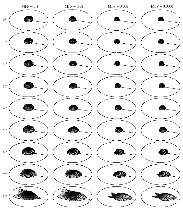
Figure 4 illustrates the effects of varying the incident light angle and mean free path (MFP) length. The incident light azimuth angle is given by the tick mark in each plot, and the elevation angle is specified to the left of each row. The surface was a Gaussian height field of 512x512 resolution with 10-12 bumps per unit length, and bump height 1-2 times the bump width. This was a very rough surface.

Figure 5 - the illuminated surface patch, with MFP length at 0.1, 0.01, and 0.001. Note the sharpening of shadows as the MFP length decreases.

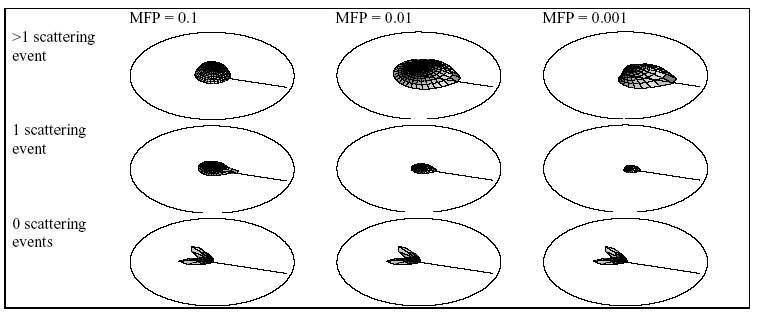
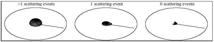
With a few exceptions, the results are unsurprising. At incident angles close to vertical, there is not much opportunity for effects depending on multiple refractions, like rays playing through multiple adjacent bumps, or effects typical of rough surfaces, such as strong retro-reflections (reflections back in the incident direction). Such reflections do appear strongly as the incident angle gets farther from vertical. At these angles the surface bumps cast shadows on each other, causing the surface to appear brighter from the angle of the light, from which no shadows are visible, and darker from other angles, as both shadowed and lit areas are visible, decreasing overall brightness. As we decrease the mean free path length, we effectively increase the opacity of the material, turning it from something like thick soup into something more resembling opaque white paint [figure 5]. As the mean free path length approaches zero, the medium becomes totally opaque and the result is a rough surface that is Lambertian. From the plots, however, we can observe that the visible differences between an MFP length of 0.001 and 0.0001 are almost nil. This is not too surprising, as even at 0.001, the distance a photon can travel in the medium before being scattered is around a hundred times smaller than the size of one bump. This is shown to be about as good as having a simple Lambertian rough surface. Decreasing this distance to 0.0001 is then an insignificant change, as far as the bump-dependent directional phenomena are concerned.

In the bottom row, the expected widening and flattening of the retro-reflection has occurred as in the Oren-Nayar model, but we can observe two “rabbit ear” reflection lobes on either side of the mirror reflection direction. A breakdown [figure 6] of this row by number of scattering events shows that the “rabbit ears” are entirely due to escaping photons that have not been scattered at all, only reflected or refracted. Because the plots for those photons are nearly identical for all path lengths, we can eliminate the possibility that refraction and transmission into the bumps is somehow contributing, as at MFP=0.1 there should be some difference due to scattering inside the bump. What is left is pure reflection, the set of photons that are mirror-reflected from the rough surface due to Fresnel reflection, which becomes more intense at glancing angles to the surface. These photons have only bounced off the sides of the bumps and been deflected very little – but never allowed to take a straight path through the bump. In the left column, the gradual “leaning” of the reflection toward glancing incident angles is replaced by a Lambertian-looking component with a noselike protuberance in the incident direction.

Figure 6 - breakdown of the 80-degree plot row of figure 4

This small, sharp retro-reflection is reminiscent of the natural heiligenschein [2] phenomenon as well as ordinary rough surface retro-reflection, as examination of the plot breakdown [figure 7] reveals that the nose is not due to multiple scattering, but is mostly the result of single scattering. The fact that it is peculiar to the MFP=0.1 plots is suspicious, as this brings the average distance a photon might travel to just about the width of a single bump. We have not found an intuitive explanation for this phenomenon, but know it has something to do with exactly one scattering event happening close to the surface, perhaps inside a bump. The retro-reflection nose was quite surprising. Decreasing the bump height by a factor of 10 produces much the same behavior but with pronounced glossy reflections (blurry, spread around the mirror reflection direction) just as previous rough-surface models predicted, with the addition of a small diffuse reflection term due to our translucent medium [figure 8]. As the bump height approaches zero, the surface becomes a plane and all notable directional phenomena disappear, leaving only Fresnel mirror reflections.

Figure 7 - breakdown of the 70-degree, 0.1 path length plot set. The nose is only present in the single scattering plot.

Figure 8 - 60-degree plot, 0.1 path length, with 1/10th bump height. Smaller bumps do not perturb Fresnel reflections as much, so they stay oriented about the mirror reflection direction.

Future Work

By fixing the absorption-to-scattering probability ratio at 1:9, we made the assumption that the ratio itself was inconsequential to the directional phenomena we were interested in. We have no strong reason to believe this is not the case, but it would not hurt to explore nonetheless.

By picking a uniform random direction at each scattering event, we were modeling isotropic scattering. Most translucent materials exhibit anisotropic scattering, which would bias selection of a new direction in favor of the current direction (forward scattering) or the direction opposite (backscattering). Scattering distribution functions have been identified for a variety of materials and could be easily incorporated into our simulator.

Choosing the standard Gaussian surface model for our rough surface let us stay within the realm of the well known. We could have chosen a pitted surface, a cracked or eroded (or simply grooved) surface, or other surface exhibiting anisotropic reflection (looking different from different azimuth angles).

Once a more complete set of variables was explored, and much more data gathered, we might begin to pick apart the observable phenomena and work toward distilling them into an easily computable analytical model for rendering purposes. At present we have only a loose collection of raw data – not nearly enough for versatile rendering. Arriving at such a model would be nontrivial at best, but it would allow a much broader range of materials to be simulated for rendering.

References